Loop Antenna
This project is a full wavelength, horizontal, loop antenna for the 40 metre Amateur Radio band. To contact local schools during the day, we needed an antenna suited to Near Vertical Incidence Skywave (NVIS) propagation. Since we were going to be using it constantly, it had to be a well-matched, resonant antenna requiring no antenna tuner. We designed it using EZNEC, by Roy Lewallan W7EL. We built it using insulated copper wire in a diamond shape, supported by egg insulators, tethered to 4 masts, each 6.5m high. We used the NanoVNA Vector Network Analyser and the NanoVNA Server application to measure the impedance, at 7.1MHz, at the end of the feedline, conveniently inside the shack. Our initial design yielded a good match with 1.3:1 SWR at 7.1MHz, but increasing to 2.4:1 at 7.0MHz and 7.2MHz. Not satisfied with that result, we used SimSmith, by AE6TY, to design a coaxial cable matching section, based on a twelfth-wavelength transmission line transformer. It turns out that by altering the lengths of the alternate 50Ω and 75Ω sections, a very wide range of complex impedances can be matched to 50Ω over a small, fixed, frequency range. The result was a perfect 1:1 match at 7.1MHz and a usable 1.6:1 match at 7.0MHz and 7.2MHz. The approach described here permits the construction of the antenna with a minimum of adjustment.
Antenna Design
We used EZNEC version 5.0 to design a 40m Horizontal Loop antenna:
- The first step was to enter the centre frequency, in this case 7.1MHz.
- EZNEC gave us the wavelength of 42m.
- We then entered details of the 4 antenna wires arranged in a diamond shape... See below.
- We connected the EZNEC 50Ω source to the end of wire 2.
- In setting the EZNEC Ground Type we have always found that Real/MININEC setting provided good correlation with the antennas we put up, while the other ground types appeared to be way off the mark.
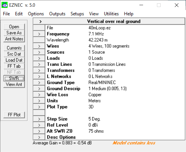
EZNEC Antenna Modelling Application
We calculated the initial wire end-point coordinates using some simple geometry:
- For a 42m wavelength each wire would be 10.5m long.
- For the wires at 45 degrees, the end-points are at: 10.5 / sqrt(2) = 7.4m
- We always use an odd number of wire segments in EZNEC.
- We chose 5.5m as the average height of the wires, as they do droop.
We used EZNEC to fine-tune the wire lengths:
- We ran the SWR prediction over the frequency band 7.0MHz to 7.2MHz.
- We then shortened or lengthened the wires to centre the minimum SWR at the centre frequency of 7.1MHz.
- We found that it was very convenient to use the Wire | Change loop size... EZNEC function to change all the wire lengths simultaneously.

EZNEC Wire Editor
When we finished adjusting the wire lengths for a minimum SWR at 7.1MHz, the predicted SWR was 1.35:1. The SWR at 7.0MHz and 7.2MHz was 2.25:1. Not too bad. The feed impedance was predicted to be 67.6Ω.
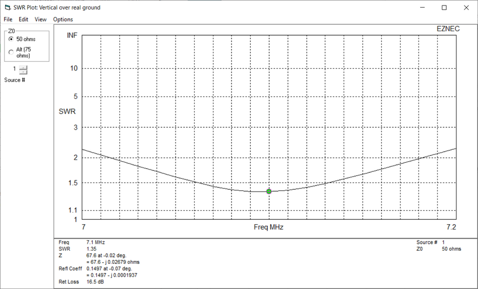
EZNEC Antenna SWR Prediction
We viewed the antenna design to check that the geometry and the feed point was correct. In this case the Y-axis pointed North and the X-axis pointed East. The image also shows the distribution of current over the wires.
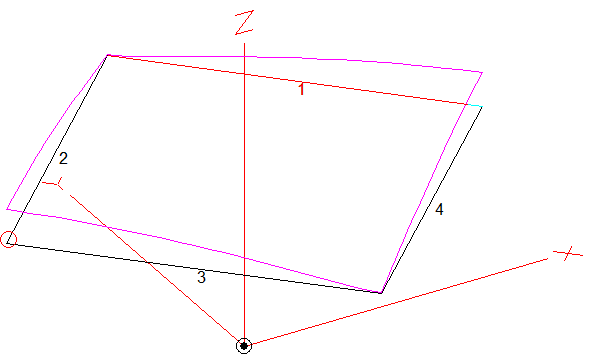
EZNEC Antenna 3D View
We checked the 3D plot of the antenna pattern. The maximum radiation is straight up with slightly more gain to the East and West.
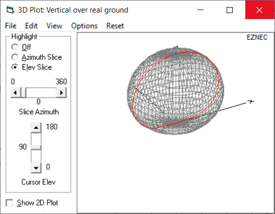
EZNEC Antenna Radiation Patern 3D Plot
We checked the East-West 2D antenna pattern.

EZNEC Antenna Radiation Pattern 2D Plot
Antenna Measurement Before Matching
We connected the NanoVNA Vector Network Analyser to the unterminated feedline, conveniently inside the shack. We then connected the NanoVNA to a Windows PC, via a USB cable, and used the Time Domain Reflectometry function of the NanoVNA Server application to measure the length of the feedline. Note: This was impossible to do manually, with a tape measure, without pulling the cable though the ceiling.
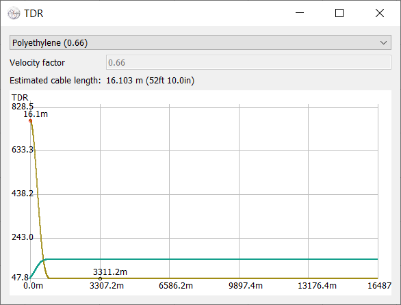
NanoVNC Server Time Domain Reflectometry Plot: Measured Feedline Length
We then connected the outside end of the 50Ω feedline directly to the loop and we raised the loop up to its full operating height. We connected a NanoVNA Vector Network Analyser to the inside end of the feedline and used it to measure the SWR.
IMPORTANT: When making antenna measurements from the end of the feedline, ensure that the feedline is in its final location with respect to the antenna, as changing the feedline route can dramatically affect the antenna impedance.
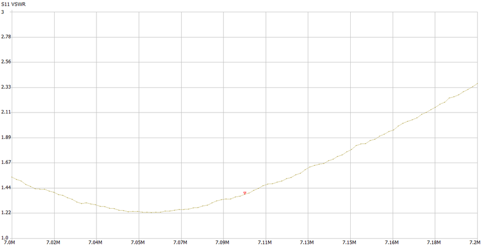
NanoVNA Server S11 VSWR Plot: Antenna SWR Before Matching
At this point, we did a check to see if a 1:1 balun was required; by looping the feedline a dozen turns and also by holding on to the feedline. There was no change in the SWR, indicating that there was negligible RF flowing on the outside of the coax. We always do this check and we install a balun only if it is required.
We measured the SWR and complex impedance of the unmatched antenna and feedline: It was 1.39:1 and 68.49Ω-j5.83Ω at 7.1MHz.
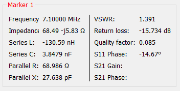
NanoVNA Server Marker 1 Data: Measured Antenna Impedance Before Matching
Matching Section Design
We then used SimSmith to design a coaxial transmission line matching section. To calculate the antenna feedpoint impedance, without having to actually measure it at the feedpoint, we used a little trick with SimSmith:
- We set the load (L) impedance in SimSmith to the measured impedance in the shack (68.49Ω-j5.83Ω).
- We then attached a simulated 50Ω transmission line (T1) to the load and set its length to a negative value equivalent to the measured length of the feedline (16.1m).
- We checked the estimated antenna feedpoint impedance at the end-point of T1: It was 61.2Ω+j16.1Ω, close to the expected 67Ω.
- We then added a 50Ω transmission line (T2) and a 75Ω transmission line (T3) to the SimSmith model. The idea was to bring the the feed impedance at the transmitter (G) to 50Ω+j0Ω.
- We adjusted the lengths of the T2 and T3 matching sections by right-clicking and dragging the (G) point to 50Ω+j0Ω.
- We were then able to read off the required section lengths of the coaxial cables: 4.52m of RG-58C/U and 1.899m of RG-59B/U.
- To make the 50Ω, RG-58C/U section we cut the existing feedline 4.52m from the antenna and installed PL-259 connectors on either side of the cut.
- We then inserted a 1.899m section of 75Ω, RG-59B/U cable terminated with PL-259 connectors on each end, using two back-to-back, SO-239 adapters.
- IMPORTANT: The 75Ω matching section must be inserted into the existing 50Ω feedline, which was used for the initial antenna measurement. Although the matching section should work with any length of 50Ω feedline, it does not take into account the additional line loss. Also, small reactive components can be amplified by connecting the 50Ω feedline. Including it in the model will also help verify the mesurements.
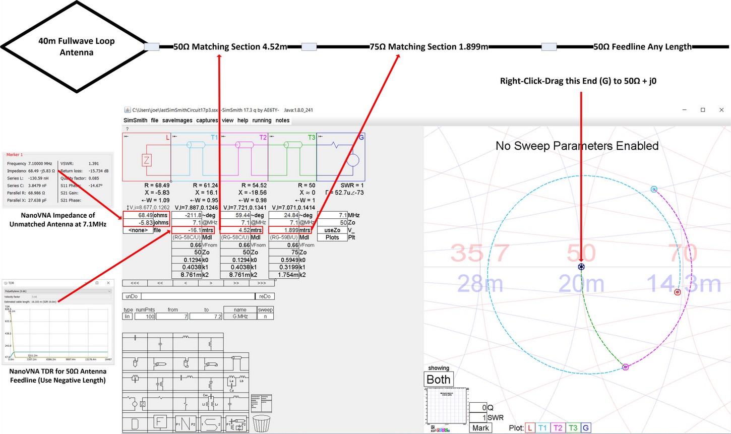
SimSmith: Antenna, Matching Sections and Transmitter Model
Antenna Measurement After Matching
We measured the matched antenna at the feed point in the shack. The results were amazing: 50.13Ω-j0.215Ω, with a near-perfect SWR of 1.005:1 at 7.1MHz and a usable SWR 1.68:1 at 7.0MHz and 7.2MHz.

NanoVNA Server S11 VSWR Plot: Antenna SWR After Matching
In this project we have shown how to design and match an antenna, using modelling and measuring tools, without the need to make reptitive, trial-and-error adjustments. Should minor adjustments be necessary, we recommend first trying to tighten or slaken the antenna tie lines. Note that reducing the height increases the antenna capacitance.
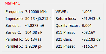
NanoVNA Server Marker 1 Data: Measured Antenna Impedance After Matching