Amateur Radio HF Communications
This activity introduces the concept of HF communications and provides practice in its use.
Introduction
High Frequency (HF) defines a segment of the Radio Frequency (RF) spectrum, located between 3MHz and 30MHz (with a wavelength of 100 metres to 10 metres, respectively). Radio communications in this band is sometimes referred to as "shortwave radio". One of the most important characteristics of HF communication is its ability to send and receive signals well beyond the usual Line-Of-Sight (LOS), over the horizon and indeed around the world! This long distance radio wave propagation is only possible because of a naturally occuring phenomenon at work high up in our atmosphere. Incredibly this miricle of nature is powered primarily by events on the surface of our sun, nearly 150 million kilometres away!
Despite this fortunate relationship between our sun and our sky, there are other phenomena that work against good HF communications and can make it quite challenging at times. The bain of many HF radio operators is of course noise, both naturally occuring sources of noise, codenamed QRN, and man-made sources, codenamed QRM.
Luckily, modern Amateur Radios work on multiple frequency bands to take advantage of the available propagation conditions and advanced modes of operation and features, which actively combat all types of noise.
This activity, which may occur over several meetings, introduces students to:
- HF Propagation;
- HF Noise; and
- HF Radio Operation.
HF Propagation
Ionospheric Layers
Circling the Earth, at an altitude of between 50 and 650 kilometres is a region of our atmosphere know as the ionosphere. Here, ultraviolet radiation from the sun ionizes molecules, liberating free electrons. Free electrons have the possibility of affecting shortwave radio communications. In some instances, they absorb the RF energy, in others they re-radiate the RF energy, sometimes causing refraction (bending) of the signals back to Earth. The concentration of ionization varies throughout the region according to some broadly-defined layers called the D, E, F1 and F2 layers. The altitude of these layers varies constantly due to the changing angle of the sun. At night, all layers start to disappear due to the lack of radiation from the sun and the recombination of the ions and electrons. The concentration of free electrons in these layers, coupled with the density of the atmosphere at different altitudes and the rate at which recombination proceeds at night, gives each of these layers different characteristics. Here is a general summary:
Characteristics of Ionospheric Layers:
- C-Layer: Very thin layer which hardly affects radio communications at all.
- D-Layer: 50-80km. Tends to absorb, not refract, RF energy travelling through this layer, in both directions, due to higher atmospheric pressure in this region.
- E-Layer: 100-125km. Little effect on radio communications, except when ionised by sporadic meteor showers.
- F1-Layer: 200-300km. Significant effect on radio communications due to lower atmospheric pressure and slower rate of recombination at night.
- F2-Layer: 300-400km. Same as F1 layer. Often merges with the F1 layer at night.
Effect of Radio Frequency
The frequency of the radio signal passing through the ionosphere also has a significant effect on HF communications: The D-Layer absorbs less RF energy at higher frequencies, but above a certain frequency, called the Maximum Usable Frequency (MUF), the radio signals pass straight through the E and F layers and are lost into space. So the MUF is usually the best frequency to use for terrestrial HF communications via the ionosphere.
Types of Ionospheric Propagation
The constantly changing radiation from the sun, the existence of the different ionospheric layers, their characteristics and the effect of the radio communications frequency used, presents various possibilities for HF communications as shown in the diagram below. Here is a general summary:
- Ground Waves: Signals from a transmitter travel only a short distance by ground wave. They can curve around the Earth and to some extent over the horizon.
- Sky Waves: Signals from a transmitter travel into the sky. The can be absorbed, refracted or pass through the ionosphere into space.
- Absorption: Signals are absorbed in the D-Layer and are not refracted back to the Earth.
- Single-Hop: Signals are refracted by the ionsophere, once, but are then attenuated by the ground or the D-Layer.
- Multi-Hop: Signals are refracted by the ionosophere, then reflected back into the ionosphere by the ground, where they are refracted again back to Earth. This can happen multiple times. Signals can travel all around the globe in all directions, even meeting themselves back at the source.
- Sporadic-E-Layer: Signals are refracted in the E-layer due to temporary ionization caused by a meteor shower.
- Ducting: Signals are refracted between layers in the ionosphere, before returning to the Earth.
- Near Vertical Incidence Skywave: Signals are virtually reflected by the ionosphere, returning to the Earth a short distance away.

Types of Ionospheric Propagation
Prediction of Ionospheric Propagation Conditions
It would be nice to know, in advance, when ionospheric propagation conditions are conducive to Amateur Radio HF Communications; just as we would like to know what the weather will be like tomorrow. Well, scientists are constantly studying this phenomenon, observing the sun and measuring its effect on our ionosphere and they have even provided many on-line tools to help us understand what is going on and, to some extent, predict what is going to happen next. They call this the study of Space Weather.
While the subject of space weather is far too extensive to cover here, let us look at some on the amazing things scientists have discovered:
- The relationship between sunspots and ionospheric conditions: The more sunspots the better the propagation!
- The existence of an 11-Year sunspot cycle: The current cycle is predicted to peak in April 2025.
- The disturbing effects of solar flares or Coronal Mass Ejection (CME) events on HF and satellite communications.
- How the magneto-sphere of the Earth creates beautiful Arora displays and stops us all frying to a crisp in deadly solar radiation.
- Published numerical indicators, called indices, which can help explain and predict ionospheric propagation.
- Solar Flare Index and Sunspot Number for solar events.
- A-Index and Planetary K-Index for fluctuations in the Earth's magnetic field.
- Proton and Electron Flux intensities for satellites in geostationary orbit.
- On-line tools and calculators
- Hourly Area Prediction and Local Area Mobile Prediction Charts showing the MUF in different areas.
- Ionogram Viewers showing the altitude and density of ionospheric layers.

SUN SPOTS

SOLAR FLARES

AURORA

SOLAR AND TERRESTRIAL DATA
SFI = SOLAR FLARE INDEX
SN = SUNSPOT NUMBER
SFI = SOLAR FLARE INDEX
SN = SUNSPOT NUMBER


HF Noise
HF Noise can best be described as anything that interferes with the signal you are trying to hear. It is the difference between speaking with someone, face-to-face, in a quiet room, and listening to them over the characteristic "snap, crackel and pop" of shortwave radio. HF Noise can be broken down into different types as follows, indeed Amateur Radio operators have more names for different types of noise than "Laplander's have for snow", or so we have heard:
HF Noise:
- Naturally Occurring Noise (QRN):
- Cosmic Noise:
- Hissing caused by white noise from the sun and the galactic centre, above 15MHz
- Swishing noises from Jupiter, around 20MHz
- Lightening Strike Noise:
- Static Crashes caused by lightning during local or remote thunder storms
- Static Electricity Noise:
- Crackling Antenna noise caused by the build-up and discharge of static electricity during a thunder storm
- Man-made Noise (QRM):
- Power Line Noise:
- Sizzling noise caused by imbalanced currents on long three-phase transmission lines.
- Buzzing noise caused by moisture or dirt on High Voltage insulators.
- Crunching noise caused by Low Voltage switching and tapping gear.
- Car Ignition Noise:
- Popcorn noise caused by spark ignition or diesel fuel injectors
- Medical Equipment Noise:
- Zipping noise cause by Diathermy equipment.
- Grinding noise cause by CAT/MRI scanning equipment
- Electrical Appliance Noise:
- Hash noise caused by motor commutator arcing.
- Whirring noise caused by motor controllers.
- Clicking noise caused by relay/contactor switch arcing.
- Electric Fence Noise:
- Rhythmic click, click, click noise caused by old types of electric fences.
- Electronic Device Noise:
- Rising buzzing noise caused by non-compliant or poorly designed switch-mode power supplies
- Chirps and Chuffs caused by computer processors.
- Birdies caused by crystal oscillators.
- Unintentional interference from other stations:
- Splattering caused by transmitter overdrive or poor ALC adjustment
- Harmonic breakthrough caused by unfiltered transmitter harmonics from lower bands
- Opposite sideband breakthrough cause by poor sideband filter role-off
- Chatter caused by DX breakthrough during rapidly changing propagation conditions
- Doubling/Stepped-On Transmissions caused by operator error
- Over-The-Horizon Radars and Ionospheric Sounders:
- Linear sweeping tones cause by vertical and oblique sounders
- Woodpecker noise caused by Russian OTHR
- Twittering noise caused by US OTHR
- Raspberry noise caused by Australian OTHR
- Illegal Radio Transmissions
- Unlicenced/Pirate Broadcast Stations
- Illegal band intrusion
HF Radio Operation
The following HF radio operation techniques can be used to take the most advantage of HF propagation conditions:
- Band Familiarisation - Knowing which bands are in use at what times.
- Time Selection - Selecting the right time to listen or call CQ.
- Band Selection - Selecting the right band to listen or call CQ on.
- Antenna Selection - Selecting the right antenna for the band and the type of propagation.
- Power Selection - Selecting the right transmitter power level.
- Monitoring DX Clusters and PSK Reporter - Checking what stations are on and which bands and which paths are in use.
The following HF radio operation techniques can be used effectively to recover HF signals in the presence of HF noise:
- Antenna Selection - Selecting and tuning the right antenna for the job.
- Frequency control - Selecting the right part of the band and being agile to move away from QRM.
- Gain Control - For SSB, max AF Gain and Min RF Gain can improve the signal-to-noise ratio.
- Attenuator/Preamp Control - Switching on these functions can also improve the signal-to-noise ratio.
- Noise Blanking - Using a noise blanker function to suppress pulse-type noise.
- Noise Reduction - Using a noise reduction function to suppress broadband noise.
- Notch Filtering - Using a Notch filter to remove nearby carriers or birdies.
- Bandpass Filtering - Selecting the right bandpass filter for the mode.
- Passband Tuning - Fine tuning the upper and lower bandpass filter cut-off frequencies for the signal.
- Headphones - Using headphones to reduce ambient acoustic noise.
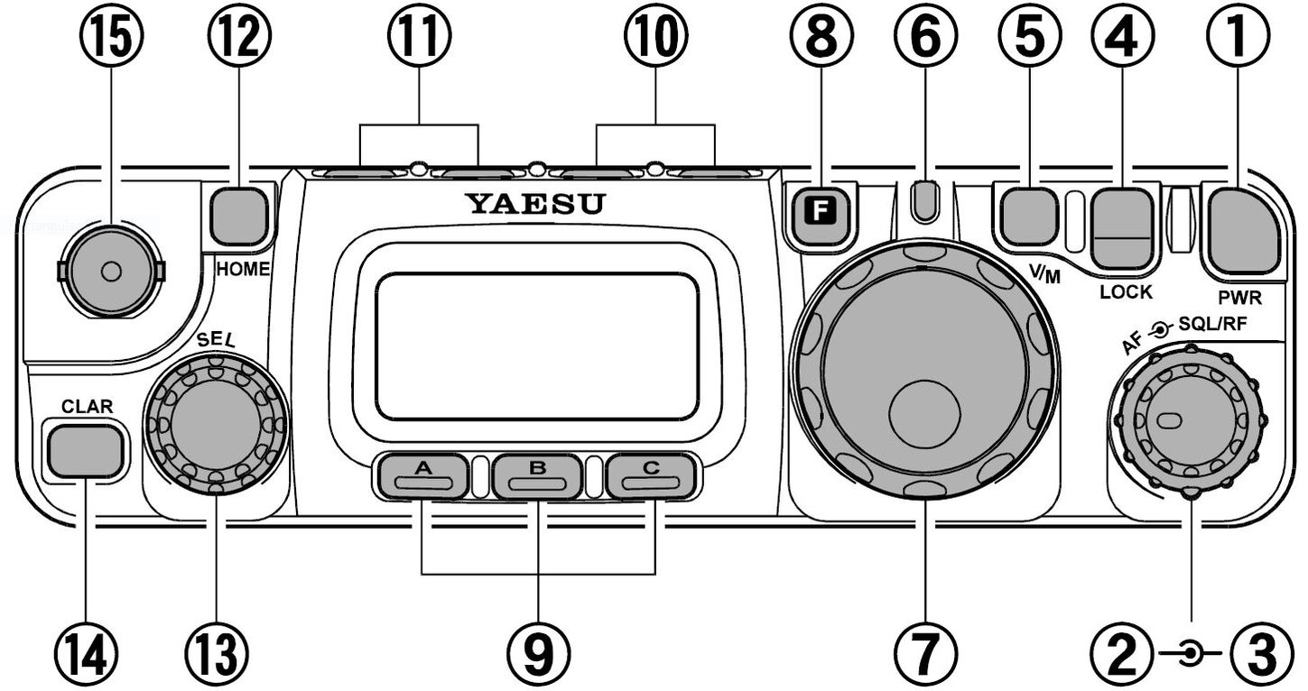
Always refer to the radio operation manual to find out the function of all the displays and controls.
Preparation
The prerequisites for this activity are: Amateur Radio Operating Procedures and Amateur Radio Operation.
You will need:
- A Power Supply for your rig.
- An Amateur Radio HF Transceiver. A low power multi-band unit like the Yaesu FT-818 is sufficient.
- An Amateur Radio HF Antenna. A 40m Half-Wave, Centre-Fed Dipole is sufficient.
- A Microphone
- A PC web browser with an Internet connection.
- The operations manual for your rig.

Activity
- Briefly present sufficient information about HF Communications and the effects of the sun on the ionospheric layers. Remind students that all HF communications is powered by the sun and only occurs on planets with an ionosphere like ours.
- Briefly present sufficient information about HF Communications and the effects of naturally-occurring (QRN) and man-made (QRM) noise.
- Briefly present sufficient information about HF Communications and the effective use of HF radio operation techniques.
- Briefly permit students to become familiar with the HF Radio operations manual.
- Turn on the HF Radio and listen to an unused frequency for a while, using SSB mode.
- Disconnect the antenna temporarily and observe that almost all of the noise is coming in from outside.
- Identify as many examples of QRN or QRM as you can. You may need to tune around to find some.
- Use the available capabilities of the HF Radio to minimise the interference.
- Tune in a selection of LX and DX SSB signals. Identify each station and its distance from your QTH by searching for the callsign on the on-line QRZ database. Is it being received by ground wave or sky wave?
- Explain (using your experience and demonstrate if you have time) what happens over a typical day and night on this band. Verify this by identifying the general location of stations at the time.
- In the late afternoon, before the band "goes long" listen carefully to see if you can hear the increasing echo-effect on local stations, caused by multi-path ionospheric refractions.
- This is the best demonstration of ionospheric propagation that we know of:
- Practice this first the day before on 40m, where this effect is most predictable.
- In the late afternoon, establish a QSO with a participating station about 300km away, near the very top of the band. You need to have 5 by 9 signals both ways.
- Use a PC to view your local ionograms over the internet every 10 minutes. Save them on the PC if you can.
- Note that the layers are receding in frequency over time: When there are no layers directly above your operating frequency, there will be no skip at all. See if you can predict when this will occur by comparing successive ionograms.
- Obtain and record accurate signal-strength reports for the remote station every few minutes and then do it constantly, when you start to loose him.
- Advise the remote station to immediately QSY -10kHz (and -10kHz again for QRM) if your signal strength drops to strength 5 or below. Both say: "QSY down 10".
- Continue this process until you are at the bottom of the band - It will take about 30 minutes.
- Note the start and stop times so you can repeat this event tomorrow.
- Congratulations: You have effectively been "Surfing the Ionosphere".


References
Homework
- Using the Space-Weather tools above plan an HF contact between two remote locations, say 1000km apart. Determine the band to use and over what times the contact will be possible.
- Using the PSK Reporter tool above, Display the two selected locations on the map. Select the Band and monitor All Signals, Sent and Received by Anyone using All Modes. Monitor the display over the predicted period. Check if communications between the two locations was possible during those times and if possible outside those times.
- Listen to HF signals using a websdr or kiwisdr station of your choice. When you hear a strange signal, see if you can identify it using sigidwiki.